Introduction
For this blog post, I decided something a bit different: I compiled all the basic knowledge i’ve gained on deep learning into a small tutorial. Hopefully it’s an interesting read.
These are the notes for day 10 of my AI/ML grind. Today’s topic: building a digit classifier.
You can also checkout these notes using my ai-ml-diary repository.
Learn basic Deep Learning concepts by building a digit classifier
I think that, as of 2026, almost everyone working with technology can acknowledge that AI will have a profound effect on society during the next 10-20 years. I know I do. This lead me to start a journey to learn more about these systems, how they work and how to best use them.
Yesterday, I wrote a neural network capable of recognizing digits from images with 95% accuracy. This was not my first ai/ml project, but it was the first one to impress me. To be honest, I thought this would be a much harder task, so it surprised me how short and intuitive the final solution was.
In fact, the project was so simple that I think it can serve as a great introduction to people who know nothing about deep learning and have never trained a neural network before. That’s what this article is! By the end of it, you should understand how neural networks work and how to train simple models with python!
Pre-Requisites
As I previously stated, this article was written for people with no prior knowledge of deep learning. However, this neither a programming tutorial nor a math tutorial. Readers are expected to be familiar with:
- The Python programming language
- Linear Algebra (Matrix Multiplication, Derivatives, …)
- Statistics (Linear Regression, …)
Notebook
The Jupyter Notebook (source code) for this article can be found on my github. I would recommend running using either Visual Studio Code or Google Colab.
An introduction to Neural Networks
The perceptron model is used to represent what happens in every node (neuron) of a neural network.
An artificial neuron takes a series of numerical inputs, transforms them using linear and non-linear operations, and outputs a singular value. This process is typically represented using the following formula:
$$ y_{prediction} = \sigma(bias + \sum_{i = 1}^n input_i * weight_i) $$
Each input is multiplied by its respective “weight” variable, with the resulting values being summed together plus the “bias” variable. This sum value is then passed through a non-linear function (like a sigmoid, for example).

Every node in a neural network works as described by the perceptron model. They are all independent and unaware of each other. The output of one node is used as the input of another. These mathematical transformations are repeated until a final value is obtained. This process is known as forward propagation.

The final prediction value output by neural network is determined by the weights associated with the inputs of each node. The goal of deep learning, is to find the set of weight values that improve a model’s accuracy as much as possible.
One way to measure a model’s accuracy is to use a loss function. A loss function compares a model’s predictions with a list of expected values, and outputs a number which indicates how far away the model was from the desired result. Depending on the problem, a different loss function is used.
The mean-squared error function is used for problems with continuous data predictions (predicting temperatures, grades, etc).
$$ 𝓛 = \frac{1}{2}(y_{prediction} - y_{expected})^2 $$
The cross-entropy error function is used for problems with categorical data predictions (change an image has a cat, what number is present in an image, etc).
$$ 𝓛 = -(y_{expected}\log(y_{prediction}) + (1-y_{expected}) log(1-y_{prediction})) $$
The lower the value of the loss function, the better the model. In order to find the the lowest possible value for the loss function, the gradient descent algorithm, a technique which uses a function’s derivative to find it’s minimum value, is used.
$$ x = x - \frac{∂y}{∂x} * learning_rate $$
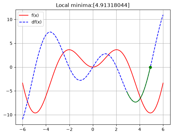
The gradient descent algorithm is applied to the weights of every node in the network. The chain rule propagates the error backward from the output through each hidden layer, in a process known as backwards propagation.
$$ w = w - \frac{η∂𝓛}{∂w} $$
The “forward propagation -> compute loss -> backwards propagation” loop is repeated until a model produces desired results.
The MNIST dataset
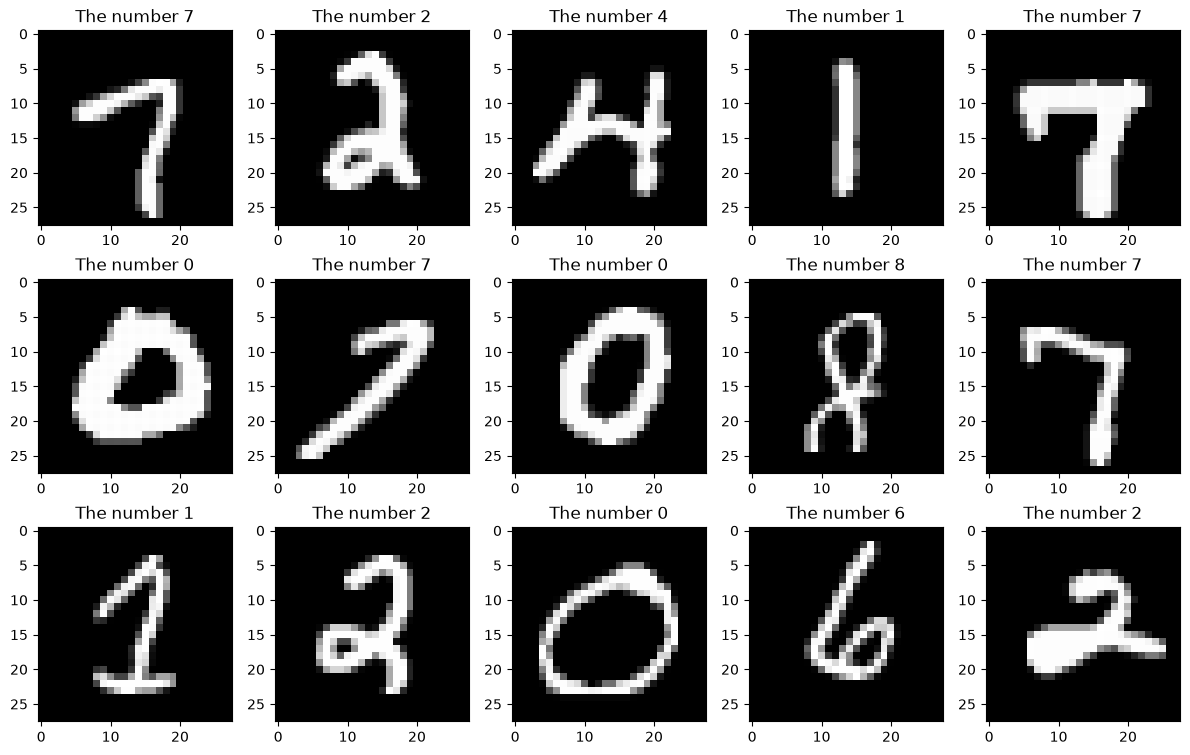
The MNIST dataset is one of the most well known datasets in ml, it’s even included in the keras library. It comes with 70 000 images of 28x28 number sprites.
from tensorflow.keras.datasets import mnist
(train_x, train_y), (test_x, test_y) = mnist.load_data()
fig, axs = plt.subplots(3, 5, figsize=(12, 8))
for ax in axs.flatten():
randimg2show = np.random.randint(0, high=train_x.shape[0])
ax.imshow(train_x[randimg2show], cmap='gray')
ax.set_title(f'The number ')
plt.tight_layout(rect=[0,0,1,0.95])
plt.show()
Building a neural network
Pytorch enables developers to build classes using different techniques. Currently, I’m a fan of writing my own classes. The process for doing this is extremely straightforward, it only requires the implementation of 3 methods: init, forward and fit.
class DigitClassifierNN(nn.Module):
    def __init__(self):
        #...
    def forward(self, x):
        #...
    def fit(self, train_data, train_labels, test_data, test_labels, learning_rate, epochs, batch_size):
        #...
The init method is used to define the model’s architecture: how many layers and how many neurons per layer. This model takes one 28x28 sprite as input, which means it need a total of 784 parameters in the input layer (one for each pixel). After the input layer, come the intermediate hidden layers. For a relatively simple problem like this, two hidden layers with 64-32 units per layer should be enough. The final output should be an array of 10 values, the chance of the input image corresponding to each digit.
def __init__(self):
    super().__init__()

    self.input = nn.Linear(784, 64)
    self.hidden1 = nn.Linear(64, 32)
    self.hidden2 = nn.Linear(32, 32)
    self.output = nn.Linear(32, 10)
In the forward method, forward progation is implemented. Each is transformed by the linear and activation functions in each layer. The standard and most widely used activation function for hidden layers in modern deep learning models is relu. This function can be used for the input and hidden layers. However, the output layer needs a function which outputs percentage values. For that, the softmax function, or variations of it, are used. Since this model has a large number of categories, the log_softmax function is used.
Log_softmax is more helpful the higher the number of categories because it massively increases the difference between the highest value and lowest values, which provides better data for the loss function.
def forward(self, x):
    x = F.relu( self.input(x) )
    x = F.relu( self.hidden1(x) )
    x = F.relu( self.hidden2(x) )
    x = F.log_softmax( self.output(x), dim=1 )
    return x
The last method is the fit method, which is where the model training actually happens. This method is slightly less intuitive than the previous ones, so I’ll divide it in steps.
The first step is to create a loss function and an optimizer. These two variables are what enable the gradient descent algorithm. The optimizer takes the value from the loss function
def fit(self, train_data, train_labels, test_data, test_labels, learning_rate, epochs, batch_size):
    # NLLLoss used over CrossEntropyLoss because of log_softmax over softmax in forward()
    loss_func = nn.NLLLoss()
    # SGD stands for Stocastic Gradient Descent
    optimizer = torch.optim.SGD(self.parameters(), lr=learning_rate)
    #...
The second step is to divide the training data into smaller batches. Iterating over small batches, as opposed to training the model on the entire dataset at once, smoothes the learning process.
    #...
    train_ldr = DataLoader(TensorDataset(train_data, train_labels), batch_size=batch_size, shuffle=False, drop_last=True)
    #...
The last step is to implement the actual training loop: forward propagation, computate loss, backwards propagation and model weight update.
  # ...
  for epoch in range(epochs):
        for i, batch in enumerate(train_ldr):
            # forward propagation
            y_hat = self.forward(batch[0])

            # computate loss
            loss = loss_func(y_hat, batch[1])

            # backprop
            optimizer.zero_grad()
            loss.backward()
            optimizer.step()
Training a neural network
After a neural network has been defined, training simply requires instantiating it and providing it with the correct input. In this case, providing the correct input involves two data transformations: flattening the data (converting 2D arrays into 1D arrays) and and normalizing it.
train_data = torch.tensor(train_x).flatten(start_dim=1)
train_data = train_data / train_data.max()
train_labels = torch.tensor(train_y, dtype=torch.long)

test_data = torch.tensor(test_x).flatten(start_dim=1)
test_data = test_data / test_data.max()
test_labels = torch.tensor(test_y, dtype=torch.long)

model = DigitClassifierNN()
model.fit(train_data, train_labels, test_data, test_labels, 0.01, 64, 32)
Results
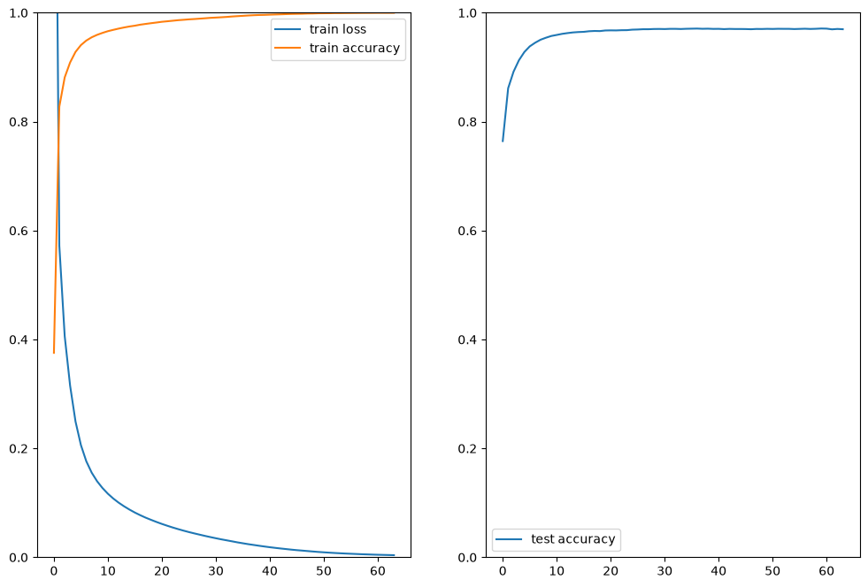
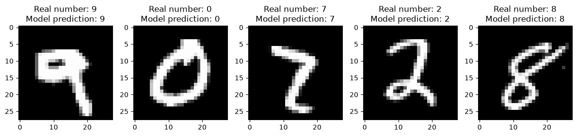
In just 64 training iterations, the mode goes to 100% accuracy on the training data and 95% accuracy on unseen test data.
Conclusion and further reading
I hope this blog post served as good introduction to the basics of deep learning. If you are interested in learning more about this topic, these are some cool resources: