ai/ml grind day 2: gradient descent

Introduction

I’ve decided that I’ll spending the next few weeks learning as much as I can about AI/ML systems. This decision has to do with some new responsabilities at my new job, and a general personal interest in the area.

I have created a github repository to store my daily notes and scripts.

I also plan to make a blog post containing the notes I put on github every day. I didn’t feel the need to write anything for day 1, since I just spent the day refreshing some high-school math, which wasn’t too interesting.

These are the notes for day 2 of my AI/ML grind. Today’s topic: the Gradient Descent algorithm.

The Gradient Descent algorithm

What is it?

In a very superficial way, this is how Deep Learning models learn:

1. Guess a solution
2. Compute the error
3. Learn from the mistakes and modify the parameters

The “error” landscape of any given problem in AI/ML has a mathematical definition. The Gradient Descent algorithm uses the derivative of the error function to find its minimum.

The algorithm

1. Initialize a random guess of the minimmum value
2. Loop over x training iterations
   1. Compute derivative at current guess minimum value
   2. Updated guess value is itself minus the derivative by the learning rate

Examples

I implemented 2 variations of the Gradient Descent algorithm: a 1-dimensional variation, and a 2-dimensional variation.

Overall, it’s a simple, elegant algorithm that feels intuitive to implement.

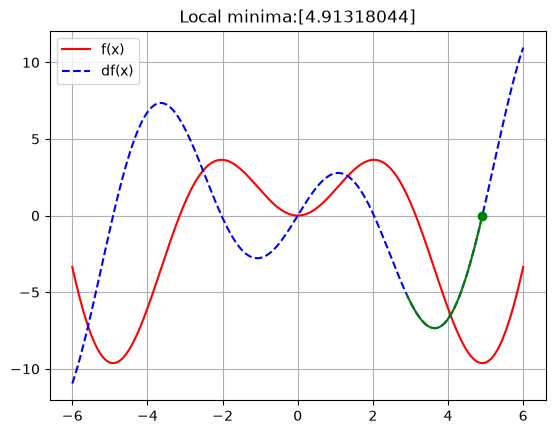
1D Gradient Descent

space_x = np.linspace(-6, 6, 500)

fx1 = sym.sin(x) * 2 * x
df1 = sym.diff(fx1, x)

fx1_func = sym.lambdify(x, fx1)
df1_func = sym.lambdify(x, df1)

localmin = np.random.uniform(space_x[0], space_x[-1], 1)
training_epochs = 200
learning_rate = 0.01

for i in range(training_epochs):
    grad = df1_func(localmin)
    localmin = localmin - grad * learning_rate

2D Gradient Descent

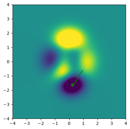
space_x = np.linspace(-4, 4, 500)

fx2 = 3*(1-x)**2 * sym.exp(-(x**2) - (y+1)**2) - 10 * (x/5 - x**3 - y**5) * sym.exp(-x**2 - y**2) - 1/3 * sym.exp(-(x+1)**2 - y**2)
df2_x = sym.diff(fx2, x)
df2_y = sym.diff(fx2, y)

fx2_func = sym.lambdify((x, y), fx2)
df2_x_func = sym.lambdify((x, y), df2_x)
df2_y_func = sym.lambdify((x,y), df2_y)

x_val, y_val = np.meshgrid(space_x, space_x)
z_val = fx2_func(x_val, y_val)

localmin = np.random.uniform(space_x[0], space_x[-1], 2)
training_epochs = 200
learning_rate = 0.02

for i in range(training_epochs):
    grad = np.array([
        df2_x_func(localmin[0], localmin[1]),
        df2_y_func(localmin[0], localmin[1])
    ])
    localmin = localmin - grad * learning_rate

In addition to these implementations, I also did some simple parametric tests, which can be found on the jupyter notebook for day 2.