robin's secret blog

Introduction

These notes should have been uploaded on 28/09, but I got really sick because of the hot summer weather hitting Portugal right now, so I skipped a day of study sessions. Sorry!

These are the notes for day 4 of my AI/ML grind. Today’s topic: implementing a neural network for linear regression.

You can also checkout these notes using my ai-ml-diary repository.

Implementing a Neural Network for Linear Regression

On day 3, I studied the inner workings of a Neural Network. I briefly explored the concepts of forward propagation, loss functions and backward propagation. Today, I decided to further explore these concepts by implementing a model capable of performing a linear regression.

Linear Regression: a machine learning and statistical method used to model the relationship between a dependent variable and one or more independent variables.

Linear Regression models work by analyzing pre-existing data, finding patterns within it, and using to predict future data. The end result for a model of this kind is a straight line that attempts to minimize prediction errors.

Generating data

In order to generate data for this experiment, I used Pytorch’s “randn” method to generate 40 pairs of (x, y) values. The x value has a significant effect on the y value.

N = 40
x = torch.randn(N, 1)
y = torch.randn(N, 1) * 0.5 + x

plt.plot(x, y, "bo")
plt.show()

Creating a Neural Network with Pytorch

Creating a neural network implies defining parameters discussed in the blog post for day 2. This neural network contains 1 input value, 1 output value and utilizes ReLU as its non-linear activation function. The learning rate is 0.5. The mean-squared error function is used for loss calculations (because this model produces numerical predictions).

ANNReg = nn.Sequential(
    nn.Linear(1, 1), # input layer
    nn.ReLU(),       # non-linear activation function
    nn.Linear(1, 1)  # output layer
)

learning_rate = 0.05
lossfunc = nn.MSELoss()
optimizer = torch.optim.SGD(ANNReg.parameters(), lr=learning_rate)

Training a Neural Network

To train the model, I implemented a standard “forward pass -> loss computation -> backprop” loop.

training_epochs = 500
losses = torch.zeros(training_epochs)

for epoch in range(training_epochs):
    # forward pass
    yHat = ANNReg(x)

    # compute loss
    loss = lossfunc(yHat, y)
    losses[epoch] = loss

    # backprop
    optimizer.zero_grad()
    loss.backward()
    optimizer.step()

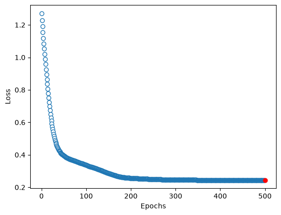
The progression of the loss value can be observed using the graph below. As expected, model performance improves exponentially until the loss value approaches zero.

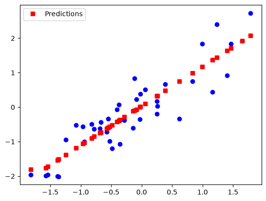
This graph showcases the difference between the model’s final predictions against the expected values. Not bad!

Further Testing

After implementing my first Neural Network, I decided to performance a simple parametric test in order to observe the effect of slop of a linear function on the loss and accuracy values of a model. I obtained these results:

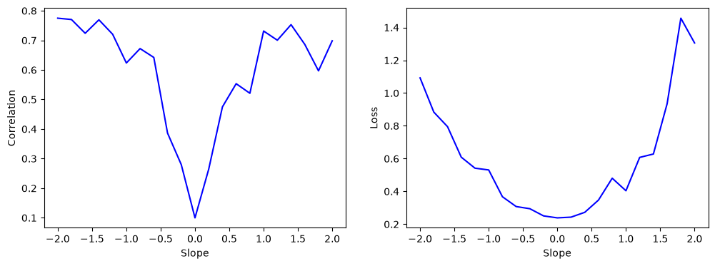
As the value of the slope approaches 0, the loss value diminishes, but model accuracy is also reduced. This might seem contradictory (a smaller loss value should indicate better model performance, in theory), however, there are explanations for this.

The losses are not normalized: they are in the scale of the data, which means a larger slope leads to higher variance in the y value. Losses can only be compared when using the same dataset, or when using different datasets that have been normalized to the same numeric range.
The closer the slope is to zero, the smaller the effect of x on y: this means the model has less information about y. Deep Learning models learn by observing the relationships between variables, the smaller the relation, the worse the model.